
Cumulative Frequency
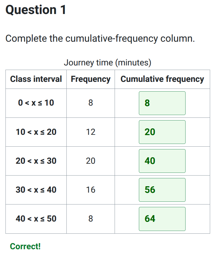
Cumulative frequency is a running total used with grouped data. It helps you estimate how many observations lie below a value and locate the middle and spread of the data.
This Higher GCSE worksheet moves from completing and reversing tables to plotting cumulative-frequency graphs at upper class boundaries. Then practise estimating medians, quartiles, interquartile ranges and frequencies, and reading backwards from a cumulative count to a data value. Jump to the questions
Practise now
Worksheet preview and key skills
Worksheet preview
Ten questions, ten marks: complete a cumulative-frequency table, recover ordinary frequencies, then plot two graphs. The second plotting question also requires you to construct the cumulative table.
Read a median, estimate quartiles and an interquartile range, find frequencies below and above thresholds, and reverse-read a value. Finally, read cumulative totals from a graph, then use successive differences to recover the class frequencies and tackle a graph whose axis extends above the actual total.
What you’ll practise
- Running totals and successive differences.
- Plotting cumulative frequencies at upper class boundaries; a lower-boundary zero start may also be included.
- Reading medians, quartiles, interquartile ranges and frequencies.
- Using the curve endpoint to identify the total frequency.
Use the interactive worksheet below, or read the Topic guide for the method and worked example.
Cumulative frequency
Complete the tables, plot the cumulative-frequency graphs and use the graphs to estimate medians, quartiles and frequencies. Each whole question is worth one mark.
Topic guide
Frequency and cumulative frequency
Ordinary frequency counts observations in one class. Cumulative frequency is the running total up to an upper class boundary: add the current frequency to all preceding frequencies.
For task times in seconds, let the classes be 10 < t ≤ 20, 20 < t ≤ 30, 30 < t ≤ 40, 40 < t ≤ 50 and 50 < t ≤ 60.
| Time (seconds) | Frequency | Cumulative frequency |
|---|---|---|
| 10 < t ≤ 20 | 6 | 6 |
| 20 < t ≤ 30 | 14 | 20 |
| 30 < t ≤ 40 | 20 | 40 |
| 40 < t ≤ 50 | 14 | 54 |
| 50 < t ≤ 60 | 6 | 60 |
For example, the third total is 6 + 14 + 20 = 40. The final cumulative frequency, 60, is the number of observations.
Reversing a cumulative table
Take successive differences, starting from zero. For cumulative totals 7, 19, 36, 52, 60, the ordinary frequencies are 7 − 0 = 7, 19 − 7 = 12, 36 − 19 = 17, 52 − 36 = 16 and 60 − 52 = 8. Check that these frequencies add to 60.
Plotting the graph
Put the measured variable on the horizontal axis and cumulative frequency on the vertical axis. For the task-time table, plot (20, 6), (30, 20), (40, 40), (50, 54) and (60, 60). You may also include the lower-boundary zero start (10, 0). It is optional, and is not the origin (0, 0): the first class begins at 10 seconds.
Use each upper class boundary, not the midpoint or the lower boundary. Join the points with a sensible smooth increasing cumulative-frequency curve (an ogive). Straight joined segments may be tolerated in exams, but this worksheet models the smooth curve convention. Its drawing questions join your points automatically; the positions of your points are marked.
Median, quartiles and interquartile range
First read the total n from the curve endpoint. The median position is n/2, the lower quartile position is n/4 and the upper quartile position is 3n/4. These are levels on the cumulative-frequency axis, not the data values you give as answers. Read horizontally from each level to the curve, then vertically down to the data axis.
For the task-time example, n = 60. The positions are 15, 30 and 45. Reading the smooth model curve gives graph estimates of a lower quartile of about 26.9 seconds, a median of 35 seconds and an upper quartile of about 43.1 seconds. Using the unrounded curve readings, the interquartile range is UQ − LQ ≈ 16.1 seconds (about 16 seconds from a graph).
Below, above and reverse reading
To estimate how many observations are below a value, read up from that value to the curve, then across to the cumulative-frequency axis. At 40 seconds in the example, the cumulative frequency is 40. For the number above 40 seconds, subtract from the total: 60 − 40 = 20 people.
For “The fastest 20 people took under how many seconds?”, start at cumulative frequency 20, read across to the curve, then down: 30 seconds. For “The slowest 6 people took longer than how many seconds?”, start at 60 − 6 = 54: the reading is 50 seconds. These are estimates from grouped data.
Checks that prevent common mistakes
- Use running totals for plotting, rather than individual class frequencies. Include every preceding class.
- Plot cumulative frequencies at the upper class boundaries. If you include a zero-frequency start, place it at the lower class boundary, not automatically at x = 0.
- Read n from the final point. An axis ending at 80 can still contain only 60 observations: the median level is then 30, not 40.
- Keep the quartile levels in order: n/4, n/2, 3n/4. Subtract data values, not cumulative counts, for the interquartile range.
- For “above”, subtract the cumulative count from n. For reverse reading, start on the cumulative-frequency axis.
- To rebuild ordinary frequencies from a graph, read cumulative totals at consecutive class boundaries and subtract the earlier total from the later one.